Coffee Cup Modeling

On Friday, we made some mathematical models of cooling and heating a cup of coffee.

Question 1: How does the cooling behavior change if we vary the parameters Rth and C? Figure this out using intuition and the above equations, and then vary these parameters in your program to confirm your conclusions.

Varying C:
Intuitively, if the material has a higher heat capacity (dE/dT), then a cup losing heat at any rate will cool down more slowly than a cup losing heat at the same rate, but with a lower heat capacity. Hence, we expect the cooling curve to be more shallow (smaller magnitude of dT/dt) as the heat capacity increases.  From the equation for dT/dt, we can also see that C appears in the denominator, confirming the idea that the curve will be shallower at higher C.
We confirmed this idea by graphing the cooling curve twice, once with C = 1000 and once with C = 1500. The C = 1500 graph had the shallower curve.

Varying Rth:
Intuitively, if there is more resistance to heat flow, heat and therefore temperature will change more slowly. This is illustrated in the equation for dT/dt in the fact that Rth is in the denominator.
We confirmed this idea by graphing the cooling curve at Rth = .85 and .95. The  Rth = .95 graph had the shallower curve.


Question 2:

Calculate a good value for P if we want our coffee to heat up to the Starbucks ideal 84°C.

Heating Simulations:
1) Bang-bang control:

Close-up of the behavior of the bang-bang control system

Overall behavior of the bang-bang control system

Bang-bang control is appropriate for many thermal systems because although it can't keep the temperature precisely at a consistent temperature, it is able to keep the temperature inside of a range that depends on the delay time of the sensor and the heater that can usually be pretty small. It could be insufficient for smaller acceptable ranges because the temperature does fluctuate up and down constantly by a small amount. 

2) Proportional control:

This approach, unlike bang-bang control, keeps the temperature very steady. However, because cooling is always happening, the temperature does not stabilize at the target temperature from which the error is calculated; it stabilizes at the temperature at which the error times the gain equals the heat loss. For this reason, the gain must be very high to get the stable temperature close to the target temperature, though it will never reach the target.

3) Bang-bang control with sensor delay:

With a sensor delay, the range of temperature gets much larger, because the coffee is allowed to cool for a much longer time before the heating kicks in each time the temperature falls below the target. There is also a delay at the start of the simulation when there is no sensor value, so the heating does not start immediately.

4) Proportional control with sensor delay:

In the proportional system, the delay causes the temperature to oscillate before stabilizing, because the heater is responding to a previous error which causes the heater to overshoot when the drink is heating and wait too long when the drink is cooling. There is also a delay at the start of the simulation when there is no sensor value, so the heating does not start immediately.

Other real-life delays could include delays between:

• the sensor recording a reading and the heater turning on
• the heater turning on and the heat reaching the coffee
• the heat reaching the coffee and the heat reaching the sensor
• the edges of the cup cooling and the center of the cup cooling (these would depend on the placement of the heat sensor). 

Modeling and Simulation: MatLab Day 1

On Wednesday, we started on Modeling and Simulation using MatLab. Most of the concepts were pretty familiar from programming, and from that one other time that I used MatLab in Physics 107. 
I will make note of some new or interesting things that we noticed while going through the exercises. 

Exercise 2.1: Fibonacci

We learned about the difference between assigning variables in the script and in the command window; we initially wanted to assign n inside the script, but the book had us assign it elsewhere to show that they variables are global across scripts and that they can be cleared and re-created in the command window (which can be monitored by typing who in the command window). 
Another useful tool is ending lines with ; to keep it from giving lots of output. 

Exercise 2.3: car_update script

Here, we used intermediate variables because we did not want one car total to update before the other. We also thought it was amusing that the book proclaims a law of "Conversation of Cars," just like in the Pixar movie. The cars reached equilibrium when .05(b)=.03(a). 

Exercise 3.1: car_loop script

The first instance of my favorite thing, the for loop. Also at this point we learned about different types of error in the book, and it was useful to see a discussion of numerical error introduced by MatLab and how it is usually a small relative error, but that we should look out for it. 

Then we learned about plotting. It is important to clear the figure (clf) and to hold to plot multiple points one after another. 

Exercise 3.2: car_loop script with plotting.  

This program produced this beautiful graph for initial values of a and b = 150

and this one for values of a and b = 10000. It appears much more "curved" than our 150-car graph because with more cars, rounding to an integer each time does not have as much of an effect. 

Exercise 3.5: fibonacci2 sequence script

This recurrently calculates Fibonacci values. We had to start with i=3 because the first two values are defined as 1. We also needed to make a special condition for n being an unsuitable number (negative). One big problem we saw was that if this NaN condition is not present, and n changes to a negative value, the program will forever return the last value it calculated before it was given a negative value, and will never alert you of the problem. Oh no!

It was also interesting to note that true and false in MatLab are just 0 and 1, no different from any other instance of 0 or 1. 

Exercise 4.6: plotting fibonacci ratios

To create this program, we learned about matrices and vectors in MatLab. Basically EVERYTHING IS A MATRIX. 

We ran the program and got out the golden ratio! 

φ fi fo fum

Baseball Simulation

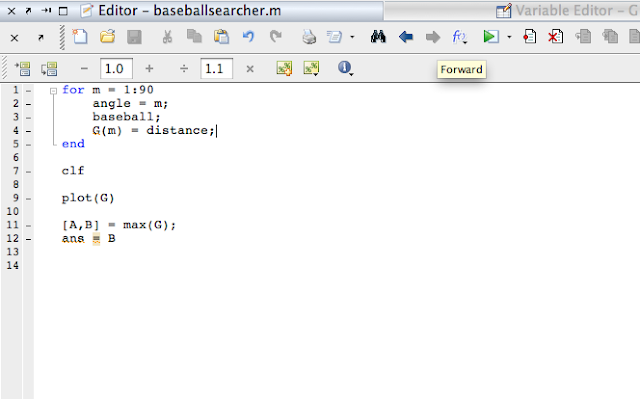
We modified the baseball simulator to change the variable "distance" to the x-distance it calculated. Then, we used this in a loop from 0 to 90 to put all the values of distance in a vector and plotted the vector. We had a big problem when we tried to use i as the index for the loop, since that is the same variable used in the baseball script itself. Once we made a new variable, we got this graph:

Using [A, B] = max(G) we found that the max = 262.5590 m at angle = 44.

Straight-Driving Conga Line

On Friday, we continued our work on proportional control by trying to combine our straight driving with our conga line program. 

First, we tried to make both components of the program proportional. We continued to have one independent wheel and one dependent wheel for the straight driving, while having the "base speed," i.e. the speed of the independent wheel, depend proportionally on input from the ultrasonic sensor. To do this, we needed two error variables: "error" being the error in the ultrasonic sensor, and "wheelerr" being the error in wheel counts. We also needed a new variable "speed" which is the power of the independent wheel based on the distance from the object. 

We also learned how to create a new block, called "valid," which outputs the value it is given unless the value is negative, in which case it outputs 0. This is useful for values given to "set power" because the power will be 100 if it is given a negative number, when we actually want the power to be 0. 

This, however, didn't work; we had the issue of, when going backward, only one wheel -- the independent wheel -- would spin, and, when returning forward, the dependent wheel would "catch up" with it. 

This program had the problem of driving backwards. We changed "set wheelerr" to a plus sign because the two wheels had opposite signs for their counts. 

Thinking this was a problem with our proportional control, we created a version that used bang-bang control for the back-and-forth motion while remaining proportional for the straight driving. This had the same problem, and we found out that it was a sign error in the power when going backwards, which was confusing us because count A increased going forward, while count C decreased going forward. We also swapped the dependent wheel's motor from C to B so that both wheels' counts increased in the forward direction. Then, we set the error to be counta-countb, but, when going backwards, the error was seThis worked!

Bang-bang control for the back-and-forth motion. The sign error was solved by making the error negative whenever the car was going backwards.  

We applied the sign fix to our proportional code, and it was also successful!

Proportional control for both the back-and-forth and straight-driving motions. 

Light Sensors

Next, in preparation for the final project, we started using the small light sensors. We decided to mount them on either side of the front of the car, so that the contrast between readings could indicate which side of the car the light was on. But, before we could get any readings, we had to get another 10Kohm resistor so that both ports could have the same resistor.

The configuration of our light sensors.

When both were connected through the same size resistor, the readings from the right and left sides were very similar, usually within 30 units.
Next, we tested the readings when a flashlight was at several positions, intending to make the car be able to follow the light of a flashlight.

However, we didn't have time to program the car. 

Driving Straight

On Wednesday, we continued to work with and inexplicably break the RDS Cricket cars. Our first task was to make a wheel return to its original position after being turned, which we had accomplished on Friday. From here, we needed to have one wheel follow the motions of the other. For this task, we wrote this program:

"followwh": By setting the error as the difference between wheel positions, Wheel A will move to match the position of Wheel B. This is a later screenshot of the program; with our first car the motor was attached to port C and will be referred to as Wheel C.  

But, we found that no matter where we turned Wheel C, Wheel A would move forward. We decided to do some tests by printing counta. Counta behaved like we would expect, with the number increasing after forward spinning and decreasing after backwards spinning. However, countc increased with both forward and backward motion. This is why Wheel A kept going forward. Robbie told us that it was an error with the car itself, and that we should just switch to Port B. However, our first car, Belle, had an existing issue with Port B. 

Hence our first car switch of the day! We got another car, named Jasmine, and we were very excited to have a nicely working car. Now, the program worked to make one wheel follow the other, so we moved to trying to get the car to drive straight. Our first idea was to use our wheel-following program, with the adjustment of setting Motor C to be on. However, we soon found that we should take away the stopping and backwards-moving parts of that program, since they would never be necessary and could be counterproductive. On Robbie's suggestion, we changed to a model of telling the car to turn either left or right, depending on whether the car was pulling to the left or to the right. 

The first program for driving straight. 

The program works by telling Wheel B to spin at a constant power, and Wheel A will speed up or slow down depending on whether the car needs to move to the left or to the right. 

Jasmine, without any modification, will turn to the left quite sharply. Running this program, it only bears slightly to the left. We couldn't see a reason within our program that would cause it to favor the left, and we even wrote a version that switched Wheel A and Wheel B, and the result was the same. To see if our program was working at least, we borrowed another car, Cinderella, which drove very nicely straight while running the program. 

At this point, Amy suggested that we try yet another car, Aurora, since Jasmine was still pulling to the left. Now, we started coming up with programs that would stop the car at the top or bottom of the ramp. First, we implemented a light sensor stop, which worked well on the way up, but the car moves so quickly going down the ramp that it passes right over the tape without registering a difference in the light sensor. We found the "stop stack" command very useful to make the car implement a final stop and stop checking or trying to move. (this program, and the ultrasonic sensor version, are included in the last picture in this post). 

Going down the ramp, but missing the tape:

To help the car stop at the bottom, we wrote the below program to use the ultrasonic, rather than the light, sensor to stop the car. 

Going up the ramp, stopping with ultrasound:

At first, it seemed to be going well, but we noticed that Aurora went really fast all the time. After noticing no change even when we changed our base speed to 20, we started testing again. After running this simple program:

Wheel B was still spinning full speed while Wheel A was stopped (as it should be). To get around this bizarre problem, we connected the motor to Port C instead. But suddenly, instead of driving straight, the car started spinning! We tested again by printing the counts and individually turning the wheels, and found that counta increased going forward and decreased backward, but countc decreased going forward and increased going backward. We changed our error expression from counta-countc to counta+countc to compensate from this. 

We also noticed, with Juliette's help, that our methods for turning right and left were identical, because the sign of the error changes depending on whether we want to turn left or right. We were able to remove the conditional and simplify the program: 

Our final collection of methods: "turn" which increases or decreases the power to Wheel A depending on whether the error is positive or negative, "drivestra" which starts the car out to drive forward and then calls another method to keep it going straight, "three" which simply keeps the car driving straight, "sonicrun" which goes straight until it is 15 units from an object, and "taperun" which goes until it passes over something dark. 

In the end, the car can go up the ramp and stop, but still goes much to fast down the ramp. Going down, it tries to compensate, but the wheel can never have more than 100 percent power and therefore cannot compensate powerfully enough at that speed. 

Proportional Control

On Friday, we worked on the new concept of Proportional Control. Instead of reacting to feedback with a simple "on or off," proportional control allows more nuanced reactions by scaling the reaction (the power level, in our case) proportionally to the error (how far the car is from an ideal state, as measured by the sensors).
Our first example of using proportional control was to revisit using the ultrasonic sensor to make the car follow a moving object like a piece of cardboard. Previously, we had a simple program of moving the car backward if the sensor read less than 15 (it was closer than 15 ultrasonic-sensor-units to the object in front of it) and forward if the sensor read more than 15, and stop if it was exactly 15. This resulted in a very choppy motion in that if you moved the leading object only a little bit, the car would surge forward and overshoot the ideal position of 15, and have to back up again (at full power).
Implementing proportional control, we introduced an "error" variable that was the reading of the sensor minus the ideal, i.e. 15. Then, the power of the car was set to be the error times an arbitrary gain variable that scales the units of error to a reasonable scale for power.
After trying this, we found that the car worked well in the forward direction, but went very slowly in the backwards direction because the sensor, as we found, will never read less than 9, and therefore the error will never be less than -6. Since this error value corresponded to such a small power, the car could never "run away" from the leading object at full speed. To solve this issue, we changed our "gain" variable and used two variables, "fgain" for forward and "bgain" for backward, and by making bgain>fgain, the car could react well to being both too close or too far away.

The program for the proportional-control object follower.

Here is a demonstration of our program:

Then we tried to implement a similar adjustment for our line follower program. Unfortunately, we couldn't even get our original line follower program to work, due to changes in the tape shade. Since we wanted the amount that the car turned to be proportional to the error, we tried to lower the power on one wheel proportionally with the error, which would make the car turn towards the lower-powered wheel. To do this, we made a new variable, dpower, which is the amount that the power decreases for the slower wheel, and set the slower wheel's power to 75-dpower. I am still not sure whether this is actually a use of proportional control, since the actual power of that wheel is not purely proportional to the error. However, I can't think of a way to structure proportional turning or "bearing" to one side where the power is 0 when the error is 0, which is a necessary result of pure proportionality.
Regardless of whether the program should have worked in theory, in practice, it was unable to "see" the line effectively and we didn't have time to work out the right numbers for the ideal range and the gain.

The proportional control line follower

Finally, we learned about the motors' ability to report their position in terms of "counts." We wrote a program that moves the axle to position 100 using both types of control, as seen below. However, we were unable to make the axle fully stop in either program, and it continued to twitch slightly back and forth after reaching the position. We tried to fix this problem by giving a range of 2-4 counts that would not cause the wheel to turn, but this was unsuccessful. For example, our proportional control program should turn the motor off if the error is between -2 and +2.

Returning the axle to position "100"

Feedback and Control: Following a Line

We are now in the unit on Feedback and Control. To get started, we were introduced to the PicoBlocks language and our car, whose name is Belle. Ashley and I worked together to learn how to use the blocks language to do many small tasks. First, we learned how to make programs that cause sounds and lights. Then, after learning how to control the motors, we could make the car move, including stopping when the car hit an object (reacting to the touch sensor), backing up, and turning in a new direction, even counting and displaying the number of times it had encountered an obstacle.

Some of the programs we wrote while exploring the PicoCricket

We also learned how to use other sensors, such as the light sensor and the ultrasound sensor. The touch sensor is the only sensor that gives a boolean (the sensor is being pressed, or it is not). The light and ultrasound sensors both give numbers, so using them as feedback requires deciding on a range of values to assign to tasks. We had a lot of trouble with our display--it would only very sporadically show any numbers at all, and sometimes would show only the number 94--but finally got a replacement cord to attach it, which solved the problem.

Armed with this knowledge, we were given the task of making the car use the light sensor to follow a white tape line along a brown background. Our first step was to see what the values were for the light sensor when it was over the tape and over the brown. Then, we tried to make the car follow the line. Our initial idea was to have the car move slowly forward as long as it was on the white line, and if it lost sight of the line, it would scan first to the right, in a series of short turns, and then back to the left. Once it found the line again, it would continue forward.

To implement this idea, we wrote many iterations of the program. The first big problem we encountered was that we could not be checking for the line (asking if the light sensor was seeing a low value) while the car was turning, unless the car kept turning indefinitely until it found the line. This was a problem because if the car was to the right of the line, and it scanned to the right first, it would turn completely around before finding the line and setting off in the wrong direction. To fix this, we changed the way it scanned to turn to the right for .1 sec, check if the light sensor saw the line, and then turn right for another short burst and check again. Because we couldn't find a way to make the control exit the loop and return to the beginning if the car found the line, we made the method recursive as seen below.

The scanning line follower

After a lot of tweaking the numbers for the power of the motors, both going straight and turning, and the interval of time that the car turned while scanning, the car was able to traverse both the straight line and the simple one-turn track, regardless of whether it started on the line or slightly to either side. However, when we put it on the big track, it was able to successfully get about halfway along and then it would suddenly stop. At first, it seemed like a battery problem, but the same thing happened after Alex changed the batteries. Apparently, because our program implemented spins instead of gradual turns, and the motors were switching quickly from forward to backward, it somehow overloaded the motors and made the machine give up halfway through. We came back after class to troubleshoot and see if we could find a way to make the car go the full distance, but we were unsuccessful. This was a very disappointing setback but we could not find another way for this method to work.

Therefore, we turned to the method of following the edge, instead of the line, causing our car to be limited to starting on a certain side of the line and causing it to be unable to traverse the sharpest turn in the course, which our first design was able to do. This program took a surprisingly short time to create, and our only setbacks were trying to find the right speed for the car to "bear" left and right so that it would not overshoot the line.

The edge follower

This program works consistently if the car starts on the curved part of the track, but overshoots the sharp curve if it starts from the straight end of the track. Juliette assured us that this was a common problem and that the program was acceptable anyway.

Obligatory Blog Post

Lego Car in Action