Modeling and Simulation: MatLab Day 1

On Wednesday, we started on Modeling and Simulation using MatLab. Most of the concepts were pretty familiar from programming, and from that one other time that I used MatLab in Physics 107. 
I will make note of some new or interesting things that we noticed while going through the exercises. 

Exercise 2.1: Fibonacci

We learned about the difference between assigning variables in the script and in the command window; we initially wanted to assign n inside the script, but the book had us assign it elsewhere to show that they variables are global across scripts and that they can be cleared and re-created in the command window (which can be monitored by typing who in the command window). 
Another useful tool is ending lines with ; to keep it from giving lots of output. 

Exercise 2.3: car_update script

Here, we used intermediate variables because we did not want one car total to update before the other. We also thought it was amusing that the book proclaims a law of "Conversation of Cars," just like in the Pixar movie. The cars reached equilibrium when .05(b)=.03(a). 

Exercise 3.1: car_loop script

The first instance of my favorite thing, the for loop. Also at this point we learned about different types of error in the book, and it was useful to see a discussion of numerical error introduced by MatLab and how it is usually a small relative error, but that we should look out for it. 

Then we learned about plotting. It is important to clear the figure (clf) and to hold to plot multiple points one after another. 

Exercise 3.2: car_loop script with plotting.  

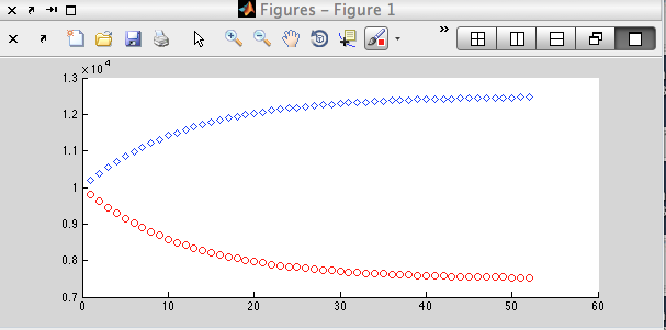
This program produced this beautiful graph for initial values of a and b = 150

and this one for values of a and b = 10000. It appears much more "curved" than our 150-car graph because with more cars, rounding to an integer each time does not have as much of an effect. 

Exercise 3.5: fibonacci2 sequence script

This recurrently calculates Fibonacci values. We had to start with i=3 because the first two values are defined as 1. We also needed to make a special condition for n being an unsuitable number (negative). One big problem we saw was that if this NaN condition is not present, and n changes to a negative value, the program will forever return the last value it calculated before it was given a negative value, and will never alert you of the problem. Oh no!

It was also interesting to note that true and false in MatLab are just 0 and 1, no different from any other instance of 0 or 1. 

Exercise 4.6: plotting fibonacci ratios

To create this program, we learned about matrices and vectors in MatLab. Basically EVERYTHING IS A MATRIX. 

We ran the program and got out the golden ratio! 

φ fi fo fum

Baseball Simulation

We modified the baseball simulator to change the variable "distance" to the x-distance it calculated. Then, we used this in a loop from 0 to 90 to put all the values of distance in a vector and plotted the vector. We had a big problem when we tried to use i as the index for the loop, since that is the same variable used in the baseball script itself. Once we made a new variable, we got this graph:

Using [A, B] = max(G) we found that the max = 262.5590 m at angle = 44.